Plotting Moment Maps

You can use the mechanisms from spectral-cube.SpectralCube to create moment maps from the modeled emission cubes. astropy and matplotlib allow for easy plotting of these images.

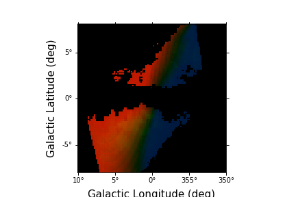
An example is to make a three color image of the Tilted Ionized gas disk of Krishnarao, Benjamin, & Haffner (2019) with red for gas with a positive mean velocity, blue for gs with a negative mean velocity, and green for the integrated intensity.

We start with computing the H-Alpha Emission Data Cube:

>>> # Import EmissionCube
>>> from modspectra.cube import EmissionCube

>>> # Use default parameters
>>> ha_cube = EmissionCube.create_DK19()

>>> ha_cube
EmissionCube with shape=(550, 128, 128) and unit=R s / km:
 n_x:    128  type_x: GLON-CAR  unit_x: deg    range:     0.000000 deg:  359.842520 deg
 n_y:    128  type_y: GLAT-CAR  unit_y: deg    range:    -7.937008 deg:    8.062992 deg
 n_s:    550  type_s: VRAD      unit_s: m / s  range:  -324408.015 m / s:  325591.985 m / s

Moments can be computed using spectral-cube.SpectralCube.moment():

>>> import astropy.units as u
>>> # Integrated H-Alpha surface brightness in Rayleighs
>>> integrated_ha = ha_cube.moment(order = 0).to(u.R)

>>> # Intensity weigted mean velocity in km/s
>>> velocity_ha = ha_cube.moment(order = 1).to(u.km/u.s)

We can construct our image array using this information and rescaling as we see fit:

>>> import numpy as np

>>> # Create RGB image array
>>> image = np.zeros((integrated_ha.shape[0], integrated_ha.shape[1] ,3))

>>> # Set Velocity Scaling:
>>> v_neg_max = -100. * u.km/u.s
>>> v_pos_max = 100. * u.km/u.s

>>> velocity_ha[velocity_ha > v_pos_max] = v_pos_max
>>> velocity_ha[velocity_ha < v_neg_max] = v_neg_max

>>> # min/max values for colors
>>> min_col = 0.25
>>> max_col = 0.75

>>> # Define Scaling Function
>>> def rescale(low, high, data):
>>>     return low + (high - low) * (data) / (np.nanmax(data))

>>> # Set scaled color intensities for velocity
>>> scaled_velocity = rescale(min_col, max_col, velocity_ha.value)


>>> # Set Integrated Surface Brightness Range
>>> int_min = 0.1 * u.R
>>> int_max = 5. * u.R

>>> integrated_ha[integrated_ha < int_min] = 0.
>>> integrated_ha[integrated_ha > int_max] = int_max

>>> # Define Scaling Function
>>> def rescale_ha(low, high, data):
>>>     return low + (high - low) * (data - np.nanmin(data)) / (np.nanmax(data) - np.nanmin(data))

>>> # Set scaled color intensities for Surface Brightness
>>> scaled_ha = rescale_ha(0.1, 0.25, integrated_ha.value)

>>> # only color places with detectable integrated surface brightness
>>> scaled_ha[integrated_ha < int_min] = 0.
>>> scaled_velocity[integrated_ha < int_min] = 0.

>>> # Set G channel
>>> image[:,:,1] = scaled_ha

>>> # Set R and B channels
>>> image[:,:,0] = scaled_velocity
>>> image[:,:,2] = -1. * scaled_velocity
>>> # Remove negative values
>>> image[image<0.] = 0.

Use astropy and matplotlib with WCS axes to plot:

>>> import matplotlib.pyplot as plt

>>> fig = plt.figure()
>>> ax = fig.add_subplot(111, projection = integrated_ha.wcs)

>>> im = ax.imshow(image)

>>> ax.invert_xaxis()
>>> ax.set_xlabel("Galactic Longitude (deg)", fontsize = 15)
>>> ax.set_ylabel("Galactic Latitude (deg)", fontsize = 15)