Custom Position-Position-Velocity Cubes
While modspectra was initially created to create HI and H-Alpha models
specific towards Krishnarao, Benjamin, & Haffner (2019), the underlying
methods can be used to create custom PPV cubes using EmissionLBV
Though the name implies an elliptical geometry, in reality, any geometry
and density distribution can be used. The underlying code relies on on
astropy.coordinates.GalacticLSR coordinate frame object to supply coordinate
and velocity information and a density grid to be provided.
We can custom create these and input them into EmissionLBV.
Start by creating a regularly spaced grid in PPV space in Galactic Coordinates:
>>> # Import statements
>>> import numpy as np

>>> # Set resolution: increase for better visuals and improved accuracy but slower
>>> # compute times
>>> nx,ny,nz = (64,64,64)

>>> # Set Data Ranges
>>> L_range = [-10,10] # Degrees Galactic Longitude
>>> B_range = [-10,10] # Degrees Galactic Latitude
>>> D_range = [6,10] # kpc

>>> # Make LBD_grid
>>> lbd_grid = np.mgrid[L_range[0]:L_range[1]:nx*1j,
>>>                     B_range[0]:B_range[1]:ny*1j,
>>>                     D_range[0]:D_range[1]:nz*1j]
This grid can be flattened and made into an astropy.coordinates.Galactic object:
>>> import astropy.coordinates as coord
>>> import astropy.units as u

>>> # Transform grid into a 3 x N array for Longitude, Latitude, Distance axes
>>> lbd = lbd_grid.T.reshape(-1,3, order = "F").transpose()

>>> # Initiate astropy coordinates.Galactic object
>>> lbd_coords = coord.Galactic(l = lbd[0,:]*u.deg, b = lbd[1,:]*u.deg, distance = lbd[2,:]*u.kpc)
These coordinates can now be transformed to different frames, such as
coord.Galactocentric or TiltedDisk. In particular, the TiltedDisk frame can be used to generically tilt any object along three axes.
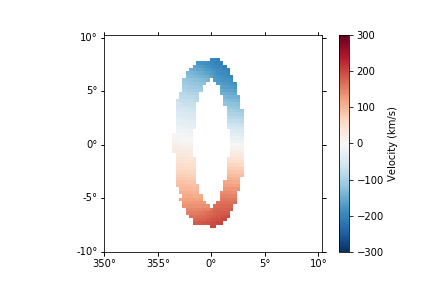
As an example, we can make a circular polar ring that is tilted 90 degrees off the plane of the Galaxy, and an inclination of 70 degrees:
>>> from modspectra.cube import TiltedDisk

>>> # Set Tilt Angles
>>> alpha = 90 * u.deg # Tilt Angle
>>> beta = 20 * u.deg # 90 - inclination
>>> theta = 0 * u.deg

>>> # Transform to GalactoCentric Coordinates first to set galcen_distance
>>> galcen_distance = 8.127 * u.kpc
>>> galcen_coords = lbd_coords.transform_to(coord.Galactocentric(galcen_distance = galcen_distance))

>>> # Transform to Tilted Disk
>>> tilted_coords = galcen_coords.transform_to(TiltedDisk(alpha = alpha, beta = beta, theta = theta))
These coordinates can now be used to define a density grid:
>>> # Reshape coordinates into grid shape
>>> # First make array of xyz coordinates in TiltedDisk Frame
>>> tilted_xyz_coords_arr = np.array([tilted_coords.x.value, tilted_coords.y.value, tilted_coords.z.value])
>>> # Reshape into grid
>>> tilted_xyz_grid = tilted_xyz_coords_arr.T.transpose().reshape(-1, nx, ny, nz)

>>> # Create a Density Grid
>>> density_grid = np.zeros_like(tilted_xyz_grid[0,:,:,:])

>>> # Define a constant density
>>> density_value = 0.5 # cm^-3
>>> # compute radial coordinate
>>> tilted_r_coord = np.sqrt(tilted_xyz_grid[0,:,:,:]**2 + tilted_xyz_grid[1,:,:,:]**2)

>>> # Set ring size masks for a ring between 0.9 kpc < r < 1.1 kpc
>>> ring_mask = (tilted_r_coord > 0.9) & (tilted_r_coord < 1.1)
>>> # Set thickness of ring as another mask in z
>>> ring_mask &= np.abs(tilted_xyz_grid[2,:,:,:]) < 0.1 # kpc

>>> # Define the density field
>>> density_grid[ring_mask] = density_value
Lastly, we can assign velocities to each coordinate. In this example, a constant angular velocity is used:
>>> # Define angular velocity by setting tangential velocity at 1 kpc
>>> v_tan_1 = 200 * u.km/u.s
>>> omega = v_tan_1 / (1. * u.kpc)

>>> # Define Tangential Velocity Field
>>> v_tan_grid = omega * tilted_r_coord*u.kpc
>>> v_tan_grid = v_tan_grid.to(u.km/u.s)

>>> # Get Velocity Vectors
>>> sin_theta = tilted_xyz_grid[1,:,:,:] / tilted_r_coord
>>> cos_theta = tilted_xyz_grid[0,:,:,:] / tilted_r_coord

>>> velocity_grid = np.zeros_like(tilted_xyz_grid)
>>> velocity_grid[0,:,:,:] = v_tan_grid.value * sin_theta # v_x
>>> velocity_grid[1,:,:,:] = v_tan_grid.value * cos_theta # v_y

>>> # Flatten Velocity to match coordinates array
>>> velocity_arr = velocity_grid.T.reshape(-1,3, order = "F").transpose() * u.km/ u.s

>>> # Define TiltedDisk Coordinates with velocity
>>> disk_coordinates = TiltedDisk(x = tilted_coords.x, y = tilted_coords.y, z = tilted_coords.z,
    v_x = velocity_arr[0,:], v_y = velocity_arr[1,:], v_z = velocity_arr[2,:],
    alpha = alpha, beta = beta, theta = theta)

>>> # Transform back to GalactoCentric with distance defined and then GalacticLSR
>>> galcen_coords_withvel = disk_coordinates.transform_to(coord.Galactocentric(
            galcen_distance = galcen_distance))

>>> lbd_coords_withvel = galcen_coords_withvel.transform_to(coord.GalacticLSR())
EmissionLBV can now be used to compute a PPV cube. It requires some
specialized arguments in the following order:
- lbd_coords_withvel: the coordinates we computed in Galactic Coordinates with Velocity Information
- density_gridin: The density grid we computed, but in order of Distance-Latitude-Longitude
- cdelt: step sizes for Longitude, Latitude, and Distance for the grid
- vel_disp: A gas velocity dispersion
- vmin/vmax: min / max velocity to compute velocity grid for
- vel_resolution: resolution of the velocity axis
- L_range: longitude range used
- B_range: latitude range used
The species keyword can be set to either ‘hi’ or ‘ha’ for HI or H-Alpha Emission. if using, speces = ‘ha’, you can also set redden = True to redden the emission values using the Marshall et al. (2006) 3D dustmaps. For this example, we will do an HI cube:
>>> # Flip density grid order
>>> density_gridin = np.swapaxes(density_grid, 0,2)

>>> Compute cdelt values
>>> dD = lbd_grid[2,0,0,1] - lbd_grid[2,0,0,0]
>>> dB = lbd_grid[1,0,1,1] - lbd_grid[1,0,0,0]
>>> dL = lbd_grid[0,1,0,0] - lbd_grid[0,0,0,0]
>>> cdelt = np.array([dL, dB, dD])

>>> # Set other parameters / args
>>> vel_disp = 9*u.km/u.s
>>> vmin = -300 * u.km/u.s
>>> vmax = 300 * u.km/u.s
>>> vel_resolution = 550

>>> # Run EmissionLBV
>>> from modspectra.cube import EmissionLBV
>>> data, wcs = EmissionLBV(lbd_coords_withvel, density_gridin, cdelt,
                            vel_disp, vmin, vmax, vel_resolution,
                            L_range, B_range, species = 'hi')
This can now be loaded as an EmissionCube to introduce the
rest of the spectral-cube pacakge tools and custom methods from this package:
>>> from modspectra.cube import EmissionCube
>>> cube = EmissionCube(data = data, wcs = wcs)

>>> cube_moment_map = cube.moment(order = 1).to(u.km/u.s)

>>> import matplotlib.pyplot as plt

>>> fig = plt.figure()
>>> ax = fig.add_subplot(projection = cube_moment_map.wcs)

>>> im = ax.imshow(cube_moment_map.data, vmin = -300, vmax = 300, cmap = 'RdBu_r')
>>> plt.colorbar(im, label = "Velocity (km/s)")